1 Introduction
Changes in climate observed over recent decades are considered to be the cause of dramatic modifications of magnitude and frequency of extreme events. The Fifth Assessment Report (AR5) of the Intergovernmental Panel on Climate Change (IPCC, 2013) has indicated a global surface temperature increase of 0.3 to 4.8 °C by the year 2100 compared to the reference period 1986-2005, with larger changes in the tropics and subtropics than in the mid-latitudes. It is expected that rising temperatures will have a major impact on the magnitude and frequency of extreme precipitation events in some regions (Barnett et al., 2006; Wilcox et al., 2007; Allan et al., 2008, Solaiman et al. 2011).
Assessment of climate change impacts and the implementation of the contemporary climate change research remains a challenge for many stakeholders and policymakers. The most likely reasons are: 1) complexity of the methods based on heavy analytical procedures and difficulties in their implementation; 2) a focus on publishing research findings under the rigorous peer review process with limited attention given to practical implementation; 3) political dimensions of climate change issues; and 4) a high level of uncertainty involved with future climate projections in presence of multiple climate models and emission scenarios. The implementation of a generic and simple web-based tool that allows users to easily consider the impacts of climate change in the form of updated IDF curves for storm water design and management is considered an effective strategy to increase climate change adaptation capacity in Canada (Sandink et al., 2016). To accomplish this task, the IDF_CC tool has been developed and has been in public use since March 2015 (Simonovic et al., 2016). This tool combines a user-friendly web-based interface with a powerful database system, and applies an efficient, sophisticated methodology for IDF curve updates.[1]
Rainfall Intensity-Duration-Frequency (IDFs) curves are typically developed by fitting a theoretical probability distribution to the annual maximum precipitation (AMP) time series. The AMP data are fitted using extreme value distributions including Gumbel, Generalized Extreme Value (GEV), Log Pearson, Log Normal, among other methods. IDF curves provide precipitation accumulation depths for various return periods (T) and different durations, typically, 5, 10, 15, 20 30 minutes, 1, 2, 6, 12, 18 and 24 hours. Longer durations may also be obtained, depending on IDF curve application. Hydrologic design of storm sewers, culverts, detention basins and other elements of storm water management systems are typically performed based on specified design storms derived from IDF curves (Solaiman and Simonovic, 2010).
The web based IDF_CC tool version 3 developed for updating IDF curves under changing climatic conditions takes the form of a Decision Support System (DSS) with three main components (Figure 1). The user interface is a GIS based component using Leaflet™, allowing clear geographical representation of hydro-meteorological stations. User information, station data, and Global Circulation Model (GCM) outputs are stored in the IDF_CC tool’s database system. Mathematical models and algorithms populate the tool’s model base.[2]
The major objectives of version 3 of the IDF_CC tool are: (i) to automate; and (ii) facilitate IDF update procedures using historical observed precipitation data and precipitation predictions from available GCMs. A repository of stations from Environment and Climate Change Canada (ECCC) is available through the user interface with complete records of historical yearly maximums. The tool also allows users to provide their own historical hydro-meteorological data, which can be used to generate locally relevant updated IDF curves. Version 3 of the tool also introduces a new dataset of ungauged IDF curves for Canada. With the new module, users can obtain IDF curves for any location in the country, especially in regions where no observations are available (i.e., ungauged locations). The new ungauged IDF curves were produced combining reanalysis data from NARR (North American Regional Reanalysis, produced by the National Centers for Environmental Prediction - NCEP) and ERA-Interim (produced by European Centre for Medium-Range Weather Forecasts - ECMRWF) datasets, available in a gridded format (see TechMan Section 3.3).
The tool interface presents IDF results in the form of tables and interactive graphs. Version 3 of the tool utilizes data from GCMs produced for Coupled Model Intercomparison Project Phase 5 - CMIP5 (IPCC, 2013) and statistically downscaled daily Canada-wide climate scenarios, at a gridded resolution of 300 arc-seconds (0.0833 degrees, or roughly 10 km) for the simulated period of 1950-2100 (PCIC, 2013) for various Representative Concentration Pathways (RCPs) (representative concentration pathways). For more information on GCMs and RCPs used with the tool, see Section 3.2 and TechMan Sections 2.3 and 2.4.
1.1 System Components
This section provides a brief description of the three major DSS components of the IDF_CC tool version 3. These components include: i) the user interface (UI); ii) mathematical models and iii) the database and GCM file repository (Figure 1).
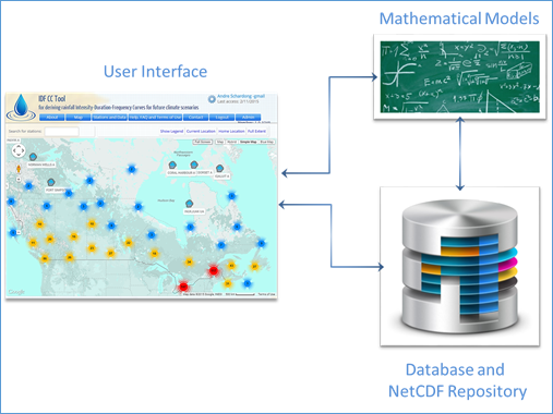
Figure 1. Major system components: user interface, mathematical models and database
1.2 Database
The following information is stored in the database:
• User information: to access the IDF_CC tool’s functionalities, users must create an account and provide data that are stored in the database, including their name, email, institution/municipality, intent of use and password.
• IDF repository of ECCC data: the IDF_CC tool’s database stores the latest hydro-meteorological station information available from ECCC stations across the country. There are approximately 700 stations throughout the country and roughly 500 of these have at least 10 years of data, which is the minimum length of time series used by ECCC to develop IDF curves for a specific station.
• User-created stations and data: any registered user can create stations and provide data for them. The type of data and input options are discussed in section 2.5.5 of this manual. User-created stations can be shared among other users registered with the IDF_CC tool.
• Original (raw) CMIP5 GCM and downscaled GCM output files: original and downscaled GCM outputs provided by IPCC PCIC (2013, refer to TechMan section 2.4) are available in netCDF format, which is widely used for storing climate data. The direct use of netCDF with the web-based IDF_CC tool is not computationally efficient and would require huge storage space. Therefore, the netCDF files are converted into a more efficient format. These converted climate data files are stored in the IDF_CC tool’s database.
• Miscellaneous files: users can upload files that are related to a specific station. The files, including text documents, spreadsheets and pdf files, are also stored within the database.
1.3 User Interface
The user interface (Figure 2) allows for management of user actions and inputs, and links with the other two DSS components: the Mathematical Models and the Database. Major components of the user interface include:
• Leaflet™: the GIS component;
• Data manipulation: functionalities that allow users to manipulate stations and data, and;
• Results visualization: functionalities that present the results to the user (tables, equations, and interactive graphs).
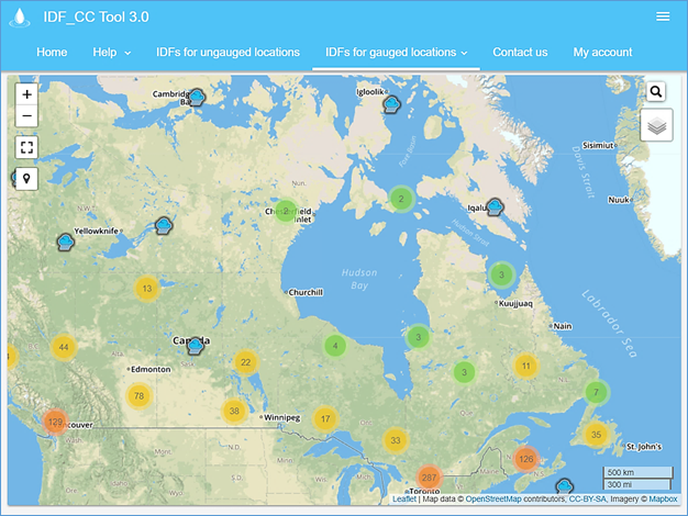
Figure 2. Screenshot of the IDF_CC tool version 3 user interface
1.4 Mathematical Models
The IDF_CC tool mathematical models are responsible for the calculations required to develop IDF curves based on historical data and incorporating GCM output data into IDF curves. Models listed bellow are used with the IDF_CC tool:
• Statistical analysis algorithms: statistical analysis is applied to fit the selected theoretical distribution to both historical and future precipitation data. The distribution applied by the tool for fitting historical data is Gumbel, which is fitted using method of moments. For future IDFs and historical data the Generalized Extreme Value (GEV) distribution is used and parameters are fitted using the L-moments method. Please refer to TechMan section 3.1 for detailed description of the Gumbel and GEV distributions.
• Optimization algorithm: an algorithm used to fit the analytical relationships (equations) to the IDF curves. For each return period (T) an equation is fitted using “Differential Evolution” optimization algorithm that is described in Storn and Price (1997) and Vasan (2008) (Appendix A). This algorithm is used to find the coefficients of the equation by minimizing the sum of the root square error of the IDF curve and calculated by the equation.
• IDF update algorithm: the Equidistant Quantile Matching (EQM) algorithm is applied to the IDF updating procedure. This algorithm combines historical observed precipitation data with data from the GCMs to develop IDF curves for future periods. A detailed description of this algorithm is presented in the TechMan section 4.
2 IDF_CC Tool Use
This section describes how to use version 3 of the IDF_CC tool. Three case studies are presented to illustrate the tool’s functionalities. The first example uses one ECCC station. The second example illustrates use of the tool for locations where ECCC data are not available. In this case, the user creates a station and inputs their own hydro-meteorological data into the tool. The third example illustrates the use of the tool where no rainfall observations are available. The IDF is estimate from the new gridded dataset of IDFs for ungauged locations incorporated in Version 3 (see section TechMan 3.3 for more details).
2.1 Creating an Account
The user must create an account before accessing full IDF_CC tool functionalities. The account is necessary to allow users to customize map locations, create stations and provide data, visualize and export historical and GCM affect IDF curve outputs. The following information is required from the user to create an account (Figure 3): Full Name, Email address, Affiliation, Occupation, Intent of Use and Password.
An email will be sent to the user with the activation code and/or activation link once the above information is provided, as shown in Figure 4 (please be sure to check the spam folder for the email sent by the tool). By clicking on the link provided, the user will activate their account. If for some reason the link does not work, the user will be required to provide an activation code when they first access the tool (Figure 5 and Figure 6).

Figure 3. Screenshot of the user account creation page
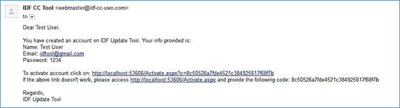
Figure 4. An example of activation email message

Figure 5. Activation page of the IDF_CC tool
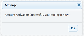
Figure 6. Message of account successfully activated and ready to use
2.2 Login and Password
After the account is created and activated, the user will be able to login using the email and password previously provided (Figure 7). The user can recover their password by using the “Recovery” option. A new password will be provided to the user by email as illustrated in Figure 8.
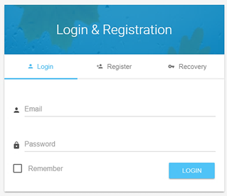
Figure 7. Login page

Figure 8. “Recover Password” screen
2.3 Main Page Description
After login, the main page is presented to the user (Figure 9). At the top portion, or header, a logo, the name of the tool, menu items, and user name are provided. The middle section is where information and maps are displayed. The footer presents information and logo from the institutions involved in the development of the IDF_CC tool.
On the top left of the header, the name of the user is presented, as shown in Figure 10. By clicking on the user’s name, the user is able to update account information as shown in Figure 11 and change passwords as shown in Figure 12.
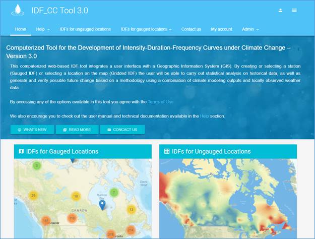
Figure 9. Main page screenshot

Figure 10. Logged user information
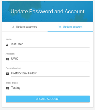
Figure 11. Updating user information
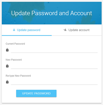
Figure 12. Updating password
2.4 Menu Options
Menu options, as presented in Figure 13, include:
· Home: description of the tool and home screen,
· Help: user manuals and additional resources,
· IDFs – ungauged locations: this option presents a map allowing the user to select any location (coordinates) in Canada to obtain the corresponding IDF information,
· IDFs – gauged locations: this option presents the map and stations from ECCC and those created by the user,
· Stations and Data: this item opens a list of stations created by the user and allows them to select data, upload companion files, share user-created stations with other users, delete and create stations. This page also allows users to see all stations from ECCC, as well as open the IDF screen,
· Help, FAQ and Terms of Use: provides access to help documents including the User Manual, TechMan, and other references, the FAQ section, and terms of use for the IDF_CC tool,
· Contact us: contact form of the tool to send comments, report bugs and other issues, and
· Admin Menu (only available to IDF_CC tool’s administrator(s)).

Figure 13. Main menu items
2.5 IDF Curves for Gauged Locations
2.5.1 Exploring Map Functionalities
The IDF_CC tool uses a GIS based map tool (LeaftLet) to assist the user in locating stations and performing other map related operations (Figure 14). This map shows all stations available from ECCC and additional user-created stations. Regions with higher station coverage are grouped (depending on the zoom level) and shown as dots. The number inside the dot is the number of stations in that region. The colours indicate station density (green for lower density, to orange for high density). As users zoom in on a specific region of the map, stations are shown individually, as presented in Figure 15. Stations created by the user are presented with an icon in green while those from ECCC are shown in blue, and stations with less than 10 years of data in grey (Figure 15).
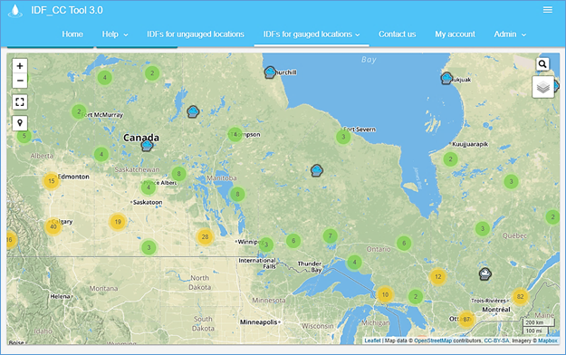
Figure 14. Screenshot with map of Canada showing stations from Environment Canada and/or user-created stations
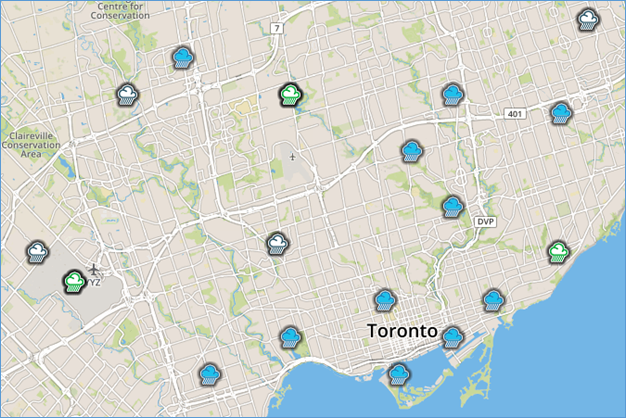
Figure 15. Stations map: Environment Canada (blue), user-created (green), and stations with less than 10 years of data (grey).
2.5.1.1 Locating an Existing Station on the Map
The stations can be visually located on the map or the user can search for stations using the search icon located in the top right corner of the map screen. As the user types in the box, the list of station names is searched and filtered based on the text provided, as in Figure 16. If the user selects one of the filtered stations, the map zooms-in and centres on the selected station (Figure 16).
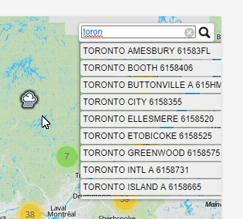
Figure 16. Additional options of the IDF_CC tool map
Additional functions are available in the top right corner over the map screen, as shown in Figure 17 and Figure 18. These functions include:
· Show/Hide Legend,
· Home Location: the IDF_CC tool allows user to set a home location by right clicking on a specific location on the map and selecting option “Set as Home Location” as shown in Figure 19. Home location is also where the map will open after login, once it is set,
·
Current Location ![]() : the IDF_CC tool will try to obtain the user’s current location
using “Geo Location.” A blue dot is placed on the location if found as in Figure 18. The user will also be asked to
allow this operation (the web browser will present this request and the message
may vary depending on the browser), and
: the IDF_CC tool will try to obtain the user’s current location
using “Geo Location.” A blue dot is placed on the location if found as in Figure 18. The user will also be asked to
allow this operation (the web browser will present this request and the message
may vary depending on the browser), and
·
Full Extent ![]() : shows the entire map of Canada as in Figure 18.
: shows the entire map of Canada as in Figure 18.
![]()
Figure 17. Additional options for the IDF_CC tool map
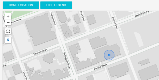
Figure 18. Current location
A right-click on the map will present a context menu (Figure 19). Options include “set as home location,” “Center map here,” “Show coordinates,” and “Create station here,” which, when selected, will open a pop-up window for creating a new station. This option will be explained later in the manual. The advantage of creating a station from the map is that it will automatically provide the coordinates and location (city and province) for the station.
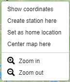
Figure 19. Context menu option on the map
2.5.1.2 Background Options for Maps
The tool provides eight different options for the map backgrounds that differ in the level of detail. The options are:
- No map: no background map is shown when this option is activated,
- OpenStreetMap: the tool’s default base map. Presents detail including street names and points of interest. The example map is presented in Figure 20,
- Clean: simplified map with only major points of interest and no labels. The example map is presented in Figure 21,
- Simplified: simplified map with only major roads and major points of interest. The example map is presented in Figure 22,
- Image: satellite images (arterial view) from ESRI © (Figure 23),
- Water colour: simplified map, with minimal details - roads and points of interest. Water bodies are presented in blue and land as light brown (Figure 24),
- Grey: Light grey map with minimum detail (Figure 25), and
- OpenTopoMap: combines topology and OpenStreetMap (Figure 26).
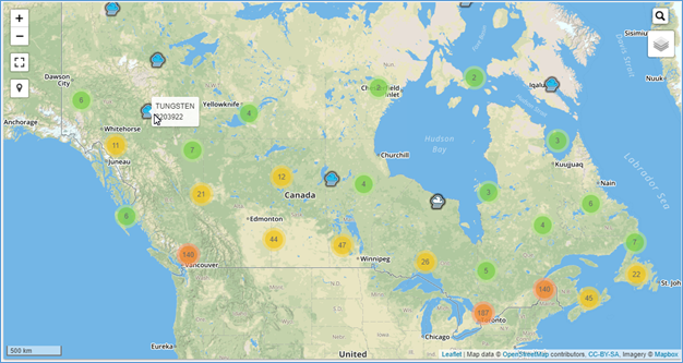
Figure 20. OpenStreeMap (IDF_CC tool’s default)
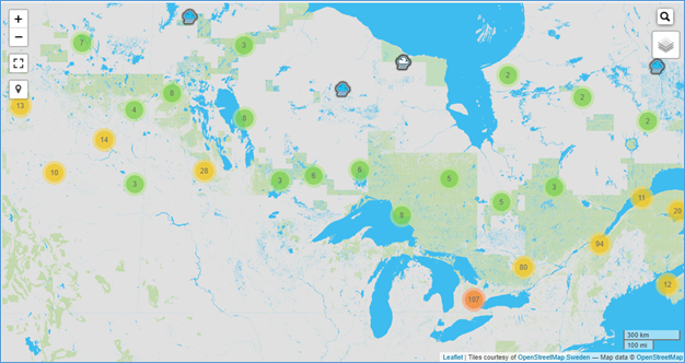
Figure 21. Clean background map
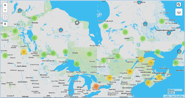
Figure 22. Simplified background map
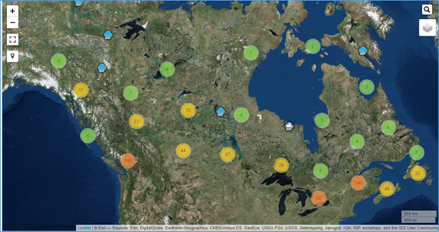
Figure 23. Arterial view background map – ESRI imagery
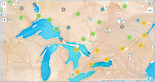
Figure 24. Water colour background map – ESRI imagery
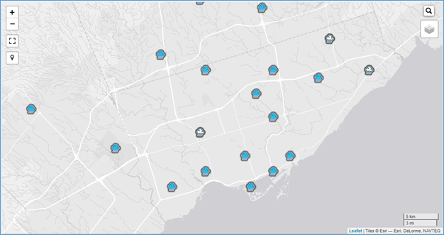
Figure 25. Grey background map – ESRI imagery
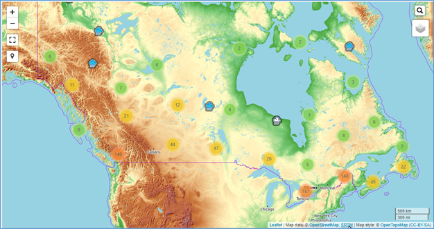
Figure 26. OpenTopoMap background map
The map also presents the source of the background map in use and the scale of the map, as shown in Figure 27.
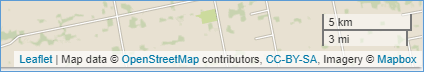
Figure 27. Map source and map scale
2.5.1.3 Creating Stations on the Map
Another function on the context menu (activated by right click on the map) is “create station here” that can be used to create a station at the selected location. This option will open a new popup window with the new station page as presented in Figure 28. Using this function, some information will be automatically filled in for the user, including latitude and longitude (in degrees), city and province (Figure 28).
Other required, user-provided information to create a station includes:
- Name (required): station name,
- Station ID (required): a unique ID has to be provided for each station. The IDF_CC tool will check if the provided ID is already in use,
- Description (optional): a description of the station,
- Sub-daily Maximums (required): the sub-daily precipitation maximums used or considered in the analysis. The defaults selected are: 5, 10, 15, 30 minutes, 1, 2, 6, 12, 24 hours,
- Additional Information (optional): any other relevant additional information about the station, and
- City and Province (optional): city and province of the station location.
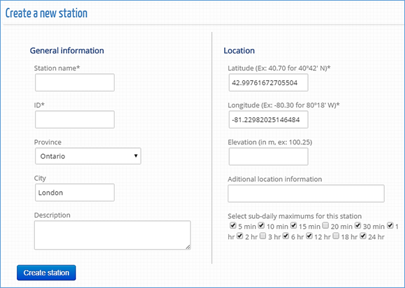
Figure 28. Creating a station on the map
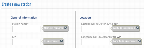
Figure 29. Required input for creating a station
The user-created station will be plotted on the map based on the provided coordinates. The coordinate system used is the World Geodetic System (WGS) also known as WGS 84 or ESPG 4326. Stations created by users are visible only to the creators. The creator can share and make the station accessible to other users within the tool. Please see Section 2.6 for more detail.
The next section explains how to provide data for a station, generate the IDFs for historical and future periods, share stations and upload files.
2.5.1.4 Legend
Legend elements are quickly described below. The legend becomes visible on the screen by selecting the “Show legend” option, as presented in Figure 30. Legend items include:
![]() Regions
with low density of stations (between 1 and 9)
Regions
with low density of stations (between 1 and 9)
![]() Regions
with medium density of stations (between 9 and 99)
Regions
with medium density of stations (between 9 and 99)
![]() Regions
with high density of stations (above 100)
Regions
with high density of stations (above 100)
![]() Stations
created by the user
Stations
created by the user
![]() Stations
from Environment Canada
Stations
from Environment Canada
![]() Stations
with less than 10 years of data
Stations
with less than 10 years of data
![]() Stations
shared with the user
Stations
shared with the user
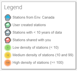
Figure 30. Legend
2.5.2 Managing Stations and Data
The user can access stations from the tool’s map view. Additionally, the “Stations and Data” option from the main menu will open a station page as shown in Figure 31. This page will show all stations created by the user and allow (i) precipitation data editing, (ii) uploading files, and (iii) sharing the station with other users. These options are presented as tabs in Figure 31.
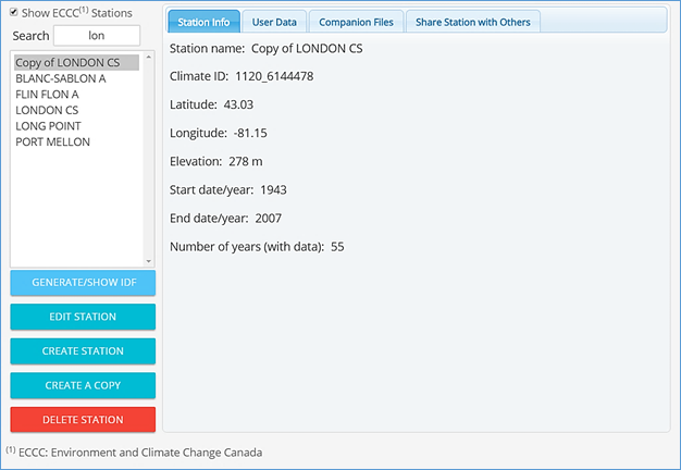
Figure 31. Station page: precipitation data editing, uploading files and sharing
The station list will only include stations created by the logged-in user and those shared with the user by other users (Figure 32). The user can search the list of stations by typing text within the search textbox above the list. A checkbox “Show ECCC Stations” allows user to see all stations in the database from ECCC, as shown in Figure 33. Stations that are shared as full access with the logged-in user will be identified with “(full access)” after the station’s name (Figure 32). If a station is shared with the logged-in use as read-only, the “(read-only)” will be added instead of “(full access)”. For more information on sharing user generated stations and station data, see Section 2.6.3.
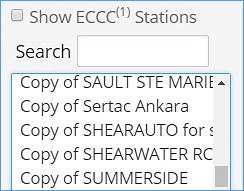
Figure 32. User-created stations
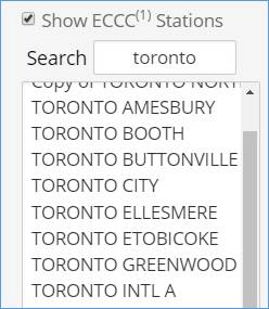
Figure 33. Stations from ECCC
Below the list of stations, additional functions are available when a specific station has been selected from the list (Figure 34), including:
- “Generate/Show IDF”: generates and shows the IDF curve and presents the page for updating IDF curves for future climate conditions. The user can also perform these functions by selecting a station on the map,
- “Edit Station”: allows user to edit station’s basic information (location, name, ID, etc.),
- “Create Station”: allows user to create a new station, and serves as an alternative to creating a station by right clicking on the map. When using this approach for creating a new station, no information about coordinates and location (city/province) will be provided and the user will have to provide this information manually,
- “Delete Station”: allows user to delete the station and all associated data, and serves as an alternative to deleting the station directly from the map, and
- “Create a Copy”: allows user to copy a station to their account. Users can copy stations from ECCC and add or modify data. Similar to user-created stations, copied stations can be deleted and edited by users.
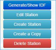
Figure 34. Options available for a selected station on list
When the selected station is from an official source (e.g., ECCC), the “Edit Station” and “Delete Station” options will not be available, as shown in Figure 35.
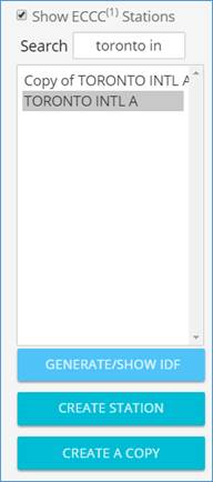
Figure 35. Users are not able to delete or edit station data for stations from official sources, including Environment Canada
Selecting one station from the list will enable the Tabs on the right side of the page (Figure 36). Each Tab is described as follows:
- Station Info: basic station information, name, coordinates, ID,
- User Data: data provided by the user. This is presented in detail in section 2.6.1.,
- Official Data: data from ECCC. No editing is possible and the yearly sub-daily precipitation maximums are presented as “read only” data to the user,
- Companion Files: allows user to upload or download supporting files (see Section 2.6.2), and
- Share Station: share station with other users registered with the IDF_CC tool (see Section 2.6.3).
![]()
Figure 36. List tabs available on the station data page.
2.5.3 Preparing and Providing Data for User-Created Stations
The IDF_CC tool allows users to provide precipitation data in two formats: daily sub-daily maximums or yearly sub-daily maximums (Figure 37). When selecting the option “Daily Maximums” the starting and ending date for the precipitation series is requested. Once the date range is defined the “Change Dates” button, when selected, will prepare the spreadsheet and allow the user to provide precipitation data within the specified range. As shown in Figure 37 the dates are shown continuously from the start to end date. Days without precipitation events can be left blank (null) or with negative values, as the IDF_CC tool’s algorithms will ignore null or negative values. It is recommended that the user prepare data using a spreadsheet processor, like Microsoft Excel™, and copy data into the IDF_CC tool by using Ctrl + C (to copy) from Excel and Ctrl + V (to paste) into the IDF_CC tool’s spreadsheet. After the data is pasted into the spreadsheet, it can be saved to the database by selecting “Save Daily Data”. Other data formats can also be used, such as formatted text files. Excel spreadsheets and text files (Figure 38) should be organized in columns, where each column represents a sub-daily maximum following the order in the IDF_CC tool’s spreadsheet (Figure 37). The user will need to provide data for sub-daily durations specified in station information (i.e., 5min, 10min ... 1hr, 2hr ... 24h), otherwise the IDF_CC tool will neither be able to fit the IDF curves nor to update them.
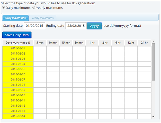
Figure 37. Editing/saving sub-daily, daily maximums
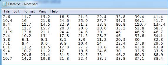
Figure 38. Formatting data in text files to paste on the IDF_CC tool’s website
When yearly sub-daily maximums are available, they can be entered into the system instead of daily data (see Figure 39). Starting and ending year are required for yearly sub-daily maximums. After defining the range and applying changes with the “Change Years” menu button, the spreadsheet will be ready to receive data. Data can also be copied using Microsoft Excel™ or formatted text files. Each column represents one sub-daily duration. Users are requested to provide data for sub-daily durations (i.e., 5 min, 10 min, 15 min, 30 min, 1hr ... 24hr) specified in the station information otherwise the IDF_CC tool will neither be able to fit the IDF curves nor update them.
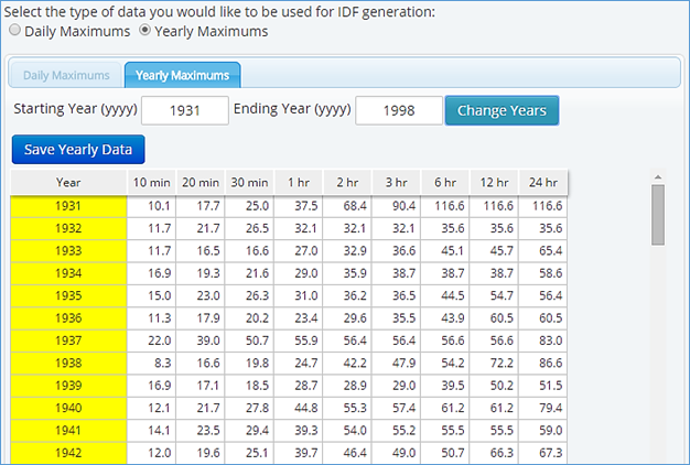
Figure 39. Saving/editing sub-daily yearly maximums
2.5.4 Companion Files
Additional files can be uploaded and downloaded for each station using the “Companion Files” tab. The types of files that can be uploaded include documents, spreadsheets, text and PDF files. These files will be available for download by the user who created the station and users with which the user has shared the station. Shared users will have either full access or read only access as specified by the user who created and shared the station (Figure 40). The file name, file size, and file type (icon) are also presented in the Tab. Users may delete uploaded documents by selecting the red “x” in the last column, if authorized to do so.
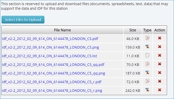
Figure 40. Uploading files
2.5.5 Sharing User-created Stations
The “Share Station” Tab allows the user to share their user-created stations with other users as illustrated in the Figure 41. There are two different levels of access: 1) “Full Access” allows the user to change data and information and view historical and updated IDFs; and 2) “Read Only” allows read only access for the station. This type of access will allow users who have been granted access to the station to view and generate updated IDFs, but will not allow these users to edit or delete station data. The station is shared by providing the email of the person with whom the user would like to share the station. If the email is associated with an account already registered within the Tool’s database, the user will only receive an email with an invitation to view the station. If the email is not registered, a temporary account will be created and on the first access the user will need to complete their registration for an account (requiring Name, Email, Affiliation, etc.). The creator of the station can also change editing/viewing permissions for users with which they have shared stations using the “Remove shared” option.
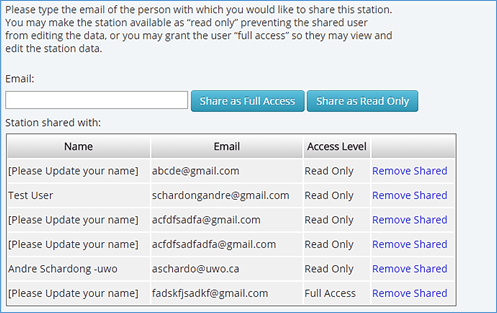
Figure 41. Sharing stations with other users
2.6 IDF Curves for Ungauged Locations
Version 3 of the IDF_CC tool includes an IDFs module for ungauged locations. This module allows the user to obtain IDF curves for any location in Canada.
The IDF_CC tool uses a GIS map tool to assist the user in selecting locations (coordinates) to obtain ungauged IDF information (Figure 42). By clicking on the map, the IDF_CC tool will select the nearest grids to the selected location and its corresponding IDF estimates, and will then interpolate and present the result to the user. An example of an IDF for a location selected form the Map is presented in Figure 43 (coordinate) and Figure 44 (IDF estimates).
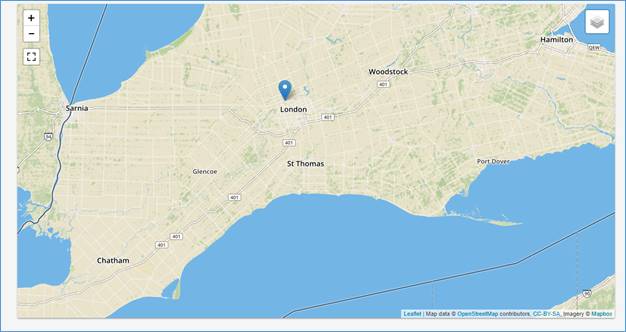
Figure 42. Screenshot with map of Canada showing stations from Environment Canada and/or user-created stations
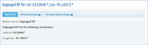
Figure 43. Example of the coordinates for the selected location from the Map
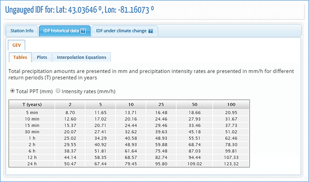
Figure 44. IDF table estimates for the selected coordinates from the Map
3 Development and Updating of IDF Curves
The IDF_CC tool allows users to simply generate and view IDF curves for any hydro-meteorological station. By selecting a station from the map or using the option “Generate/Show IDF” option described in the previous section, a new pop-up window appears (Figure 45). The first tab (“Station Info”) presents the name, ID, location and information and record lengths for the station. The other two tabs, “IDF, historical data” and “IDF under climate change” are described in sections 3.1 and 3.2, respectively.
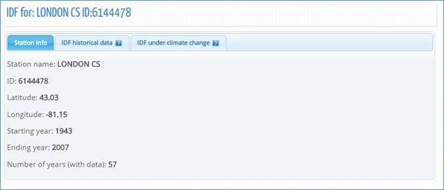
Figure 45. IDF_CC tool page with station information, historical and future IDF
3.1 IDF Curves for Gauged Locations
When the user requests to view an IDF curve for a station, the IDF_CC tool triggers a calculation process using mathematical models in the background. When the “IDF, historical data” tab is selected, an IDF curve based on the observed historical precipitation data available is presented to the user. The background data analysis steps are as follows:
1) Read and organize data from the database for the selected station.
2) Data analysis (ignore negative and zero values) and extraction of yearly maximums.
3) Calculate statistical distributions parameters for GEV and Gumbel using L-moments and method of moments, respectively. For more details on Gumbel distribution please refer to TechMan section 3.1.1 and 3.1.2.
4) Calculate IDF (please refer to TechMan section 2.1 and 3.1 for more detail).
5) Fit interpolated equations to the IDF curve using optimization algorithm (Differential Evolution): refer to Storn and Price (1997) and Vasan (2008) for more details on Differential Evolution optimization (available in Appendix A).
6) Organize data for display (tables, plots, and equations).
After the calculation steps are completed the IDF information is presented in the form of tables, total precipitation, intensity graphs and the fitted equation. These results are presented by selecting “IDF, historical data” Tab as in Figure 46. The IDF is fitted to the historical data using GEV and Gumbel distribution and results are presented in the following forms:
1) Tables: the IDFs are presented in traditional tabular format with duration (in minutes and hours) and return period (T) as in Figure 46. Both total precipitation (Figure 46 in mm and intensity (Figure 47) in mm/h are presented and the user can toggle between these two options.
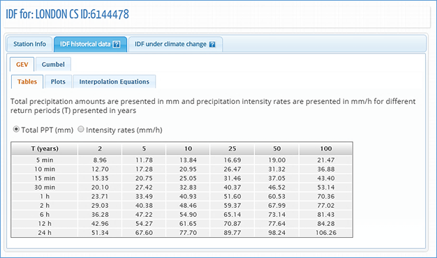
Figure 46. Total precipitation (in mm) IDF table
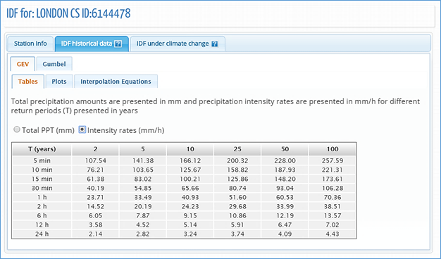
Figure 47. Rainfall intensity (in mm/h) IDF table
2)
Plots: the plots or graphs are also presented as Total Precipitation (in
mm) and Intensity (mm/h) as shown in Figure 48 and Figure 49, respectively. The user can hide
or show the IDF curve for each return period by clicking on individual return
periods in the legend below the graph. A zoom option is also available and is
performed by dragging out a rectangle in the chart with the mouse pointer. The
map will enlarge the selected area (Figure 50). The “Reset zoom” option will
revert the initial zoom level (Figure 48). By hovering the mouse pointer over dots, the user can view
precipitation, intensity and duration values for each point on the plot. The
dots are calculated IDF values and the lines are plotted using the fitted equation
that is presented under the “Interpolation Equation” tab. A button on the top
left of the plot (![]() )
allows user to print and export/download the graph to images file (Figure 51).
)
allows user to print and export/download the graph to images file (Figure 51).
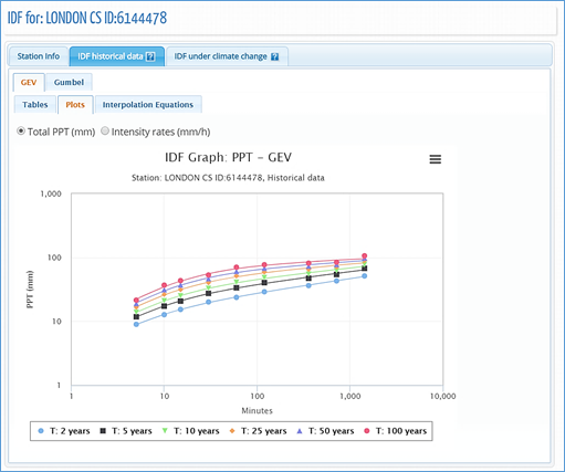
Figure 48. Total precipitation (in mm) IDF graph for different return periods
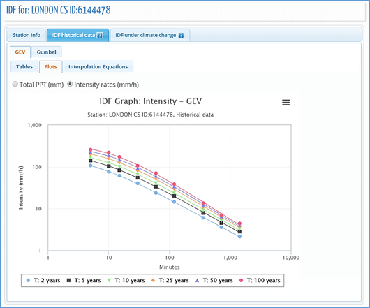
Figure 49. Rainfall intensity (in mm/h) IDF graph for different return periods
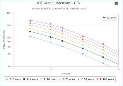
Figure 50. Zooming on a plot and resetting zoom level
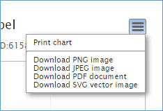
Figure 51. Printing and exporting a plot as image
3) Interpolation Equations: an optimization algorithm is used to fit equations to the calculated IDF values. The equations are presented under the “Interpolation Equations” Tab as shown in Figure 52. Three coefficients A, B and t0 are calculated by the optimization algorithm for each return period (T) and presented as a table in Figure 52. This equation can be applied as a fast method for interpolation and calculation of design storms.
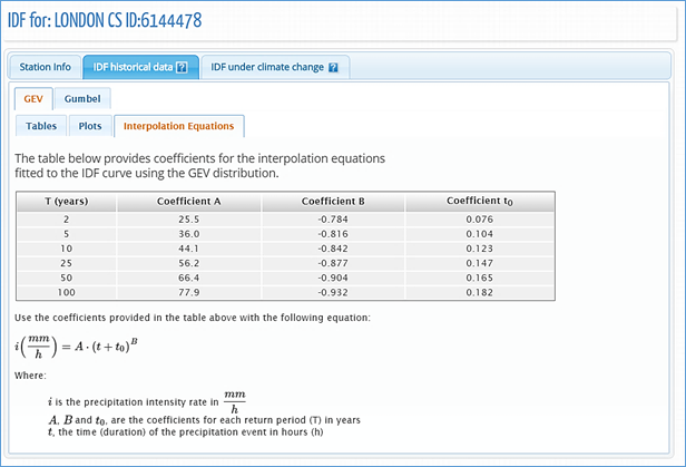
Figure 52. Fitted IDF equation to historical precipitation data
3.2 IDF Curves for Ungauged Locations
A new dataset of ungauged IDF curves for Canada is available in version 3 of the IDF_CC tool. With the new module, users can obtain IDF curves for any location in the country, including regions where no observations are available. The IDF estimates are calculated according to the methodology described in TechMan section 3.3. For a selected location from the map the IDF_CC tool will present the ungauged IDFs in a similar format as the ones based on gauged observations (describe on item 3.1).
The user will select the location (coordinates) from the Map, and based on the input, the IDF_CC tool will identify the nearest grids, and present the IDF curves. Figure 53 presents a screenshot with the coordinates of the selected location. The elements are presented in similar format to the gauge-based IDFs: tables (Figure 54), interactive graphs (Figure 55) and the fitted equation (Figure 56).

Figure 53. IDF_CC tool page with the coordinates of the selected location for the ungauged IDF
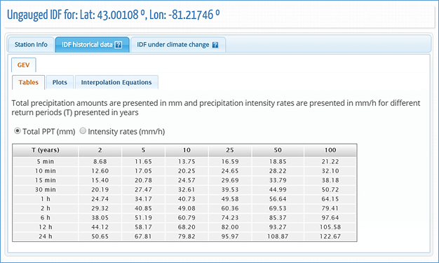
Figure 54. Total precipitation (in mm) IDF table for the selected coordinates
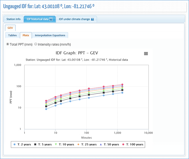
Figure 55. Total precipitation (in mm) IDF graph for different return periods
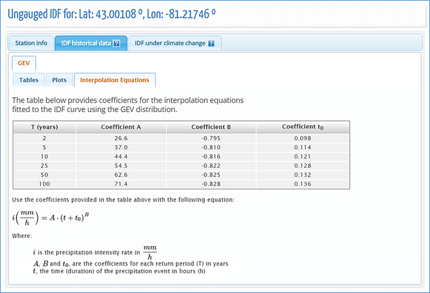
Figure 56. Fitted IDF equation to precipitation data for the selected location
3.3 Updated IDF Curves Under Climate Change
By selecting the “IDF under climate change” tab, the user can generate IDF curves that account for future climate conditions. To generate IDFs for future climate, the user can select all models (ensemble option) or an individual GCM and projection period (Figure 57). There are 9 bias corrected models (Table 1) and 24 raw GCMs (Table 2) resulting in a total of 33 GCM datasets available with the IDF_CC tool. The dataset used for the updating procedure is a choice of the user: “Bias Corrected” or “Raw GCMs”. The available range for the future time period is 2006 to 2100 (Step 1 in Figure 57). The updating procedure applies for both gauged and ungauged IDFs.
With respect to GCM selection, to generate IDF curves that account for climate change, the user has two options: select all models (ensemble option), or select any model from the list of GCMs provided with the tool (Step 2 in Figure 57). The users are encouraged to test different models due to uncertainty associated with climate modeling. The climate modelling community does not “compare” global climate models to identify superior/inferior models for specific locations. Thus, users should not that there is no “right” GCM for any given location. Users are provided access all available models in the IDF_CC tool to allow them to understand uncertainty associated with potential climate change impacts.
The following steps are performed by the IDF_CC tool to update IDF curves for future climate. Please see TechMan section 4 for more information on each of the steps:
1) Extract precipitation data series from GCM grid points for the selected station (e.g., using BCCAQ with the Canadian CanESM2 model),
2) Organize data and extract yearly maximums,
3) Apply Equidistant Quantile Matching (EQM) algorithm (refer to TechMan section 4.1 and 4.2),
4) Estimate distribution parameters and calculate IDFs for each future climate scenario (RCPs),
5) Generate median IDF from the results of step 4 for each RCP, and
6) Organize data for display (tables, plots, and equations, uncertainty range plot).
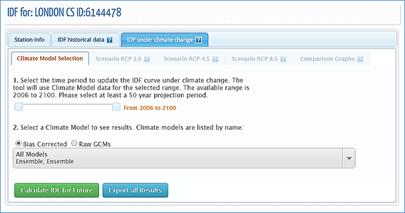
Figure 57. Selection of the CGM model and projection period
The Fifth Assessment Report (AR5) (IPCC, 2013) provides four RCP scenarios: RCP2.6, RCP 4.5, RCP 6.0 and RCP 8.5. The following definitions are directly adopted from AR5 and the RCPs are briefly described below (refer to TechMan section 2.3 for more details):
· RCP 2.6: pathway where radiative forcing peaks at approximately 3 W m–2 before 2100 and then declines;
· RCP 4.5 and RCP 6.0: two intermediate stabilization pathways in which radiative forcing is stabilized at approximately 4.5 W m–2 and 6.0 W m–2 after 2100;
· RCP 8.5: high pathway for which radiative forcing reaches greater than 8.5 W m–2 by 2100 and continues to rise for some time.
The future emission scenarios used in the IDF_CC tool are RCP 2.6, RCP 4.5 and RCP 8.5. RCP 2.6 represents a low greenhouse gas concentration scenario, followed by RCP 4.5 as an intermediate scenario and RCP 8.5 as a high concentration scenario. The RCP 4.5 scenario was selected over RCP 6.0 as an intermediate scenario largely because more GCMs have results for RCP 4.5 than RCP 6.0.
Table 1 – Bias corrected climate models list used with the IDF_CC Tool – PCIC (2013)
|
Bias Correction Methods |
Model |
|
Country |
Centre Name |
Original (Lon. vs Lat.) |
Bias corrected (Lon. vs Lat.) |
|
BCCAQ |
CanESM2 |
|
Canada |
Canadian Centre for Climate Modeling and Analysis |
2.8 x 2.8 |
0.0833 x 0.0833 |
|
BCCAQ |
CCSM4 |
|
USA |
National Center of Atmospheric Research |
1.25 x 0.94 |
|
|
BCCAQ |
CNRM-CM5 |
|
France |
Centre National de Recherches Meteorologiques and Centre Europeen de Recherches et de Formation Avancee en Calcul Scientifique |
1.4 x 1.4 |
|
|
BCCAQ |
CSIRO-Mk3-6-0 |
|
Australia |
Australian Commonwealth Scientific and Industrial Research Organization in collaboration with the Queensland Climate Change Centre of Excellence |
1.8 x 1.8 |
|
|
BCCAQ |
GFDL-ESM2G |
|
USA |
National Oceanic and Atmospheric Administration's Geophysical Fluid Dynamic Laboratory |
2.5 x 2.0 |
|
|
BCCAQ |
HadGEM2-ES |
|
United Kingdom |
Met Office Hadley Centre |
1.25 x 1.875 |
|
|
BCCAQ |
MIRCO5 |
|
Japan |
Japan Agency for Marine-Earth Science and Technology |
1.4 x 1.41 |
|
|
BCCAQ |
MPI-ESM-LR |
|
Germany |
Max Planck Institute for Meteorology |
1.88 x 1.87 |
|
|
BCCAQ |
MRI-CGCM3 |
|
Japan |
Meteorological Research Institute |
1.1 x 1.1 |
Table 2 – Climate models list used with the IDF_CC Tool – IPCC (2015)
|
Country |
Centre Acronym |
Model |
Centre Name |
Number of Ensembles (PPT) |
GCM Resolutions |
|
(Lon. vs Lat.) |
|||||
|
China |
BCC |
bcc_csm1_1 |
Beijing Climate Center, China Meteorological Administration |
1 |
2.8 x 2.8 |
|
China |
BCC |
bcc_csm1_1 m |
Beijing Climate Center, China Meteorological Administration |
1 |
|
|
China |
BNU |
BNU-ESM |
College of Global Change and Earth System Science |
1 |
2.8 x 2.8 |
|
Canada |
CCCma |
CanESM2 |
Canadian Centre for Climate Modeling and Analysis |
5 |
2.8 x 2.8 |
|
USA |
CCSM |
CCSM4 |
National Center of Atmospheric Research |
1 |
1.25 x 0.94 |
|
France |
CNRM |
CNRM-CM5 |
Centre National de Recherches Meteorologiques and Centre Europeen de Recherches et de Formation Avancee en Calcul Scientifique |
1 |
1.4 x 1.4 |
|
Australia |
CSIRO3.6 |
CSIRO-Mk3-6-0 |
Australian Commonwealth Scientific and Industrial Research Organization in collaboration with the Queensland Climate Change Centre of Excellence |
10 |
1.8 x 1.8 |
|
USA |
CESM |
CESM1-CAM5 |
National Center of Atmospheric Research |
1 |
1.25 x 0.94 |
|
E.U. |
EC-EARTH |
EC-EARTH |
EC-EARTH |
1 |
1.125 x 1.125 |
|
China |
LASG-CESS |
FGOALS_g2 |
IAP (Institute of Atmospheric Physics, Chinese Academy of Sciences, Beijing, China) and THU (Tsinghua University) |
1 |
2.55 x 2.48 |
|
USA |
NOAA GFDL |
GFDL-CM3 |
National Oceanic and Atmospheric Administration's Geophysical Fluid Dynamic Laboratory |
1 |
2.5 x 2.0 |
|
USA |
NOAA GFDL |
GFDL-ESM2G |
National Oceanic and Atmospheric Administration's Geophysical Fluid Dynamic Laboratory |
1 |
2.5 x 2.0 |
|
USA |
NOAA GFDL |
GFDL-ESM2M |
National Oceanic and Atmospheric Administration's Geophysical Fluid Dynamic Laboratory |
|
2.5 x 2.0 |
|
United Kingdom |
MOHC |
HadGEM2-AO |
Met Office Hadley Centre |
1 |
1.25 x 1.875 |
|
United Kingdom |
MOHC |
HadGEM2-ES |
Met Office Hadley Centre |
2 |
1.25 x 1.875 |
|
France |
IPSL |
IPSL-CM5A-LR |
Institut Pierre Simon Laplace |
4 |
3.75 x 1.8 |
|
France |
IPSL |
IPSL-CM5A-MR |
Institut Pierre Simon Laplace |
4 |
3.75 x 1.8 |
|
Japan |
MIROC |
MIROC5 |
Japan Agency for Marine-Earth Science and Technology |
3 |
1.4 x 1.41 |
|
Japan |
MIROC |
MIROC-ESM |
Japan Agency for Marine-Earth Science and Technology |
1 |
2.8 x 2.8 |
|
Japan |
MIROC |
MIROC-ESM-CHEM |
Japan Agency for Marine-Earth Science and Technology |
1 |
2.8 x 2.8 |
|
Germany |
MPI-M |
MPI-ESM-LR |
Max Planck Institute for Meteorology |
3 |
1.88 x 1.87 |
|
Germany |
MPI-M |
MPI-ESM-MR |
Max Planck Institute for Meteorology |
3 |
1.88 x 1.87 |
|
Japan |
MRI |
MRI-CGCM3 |
Meteorological Research Institute |
1 |
1.1 x 1.1 |
|
Norway |
NOR |
NorESM1-M |
Norwegian Climate Center |
3 |
2.5 x 1.9 |
3.4 Viewing and Exploring Results
Upon completion of the IDF update calculations, the results are presented in the form of tables, total precipitation, rainfall intensity graphs and uncertainty range graphs. These results are presented for each RCP future scenario: 2.6, 4.5 and 8.5. Each RCP scenario is displayed as a set of Tabs as shown in Figure 58.
Updated IDF curves for future climate conditions for all three RCPs are presented as tables, plots and uncertainty ranges, as described here:
1) Tables: IDF information is presented in the traditional table format for all durations (in minutes and hours) and return periods (T) as illustrated in Figure 58. Both total precipitation in mm (Figure 58) and rainfall intensity in mm/h (Figure 59) are available and the user can toggle between these two options using the available radio buttons. The IDF curves presented in Figure 58 and Figure 59 are a median from all models selected for each emission scenario (see TechMan section 2.3).
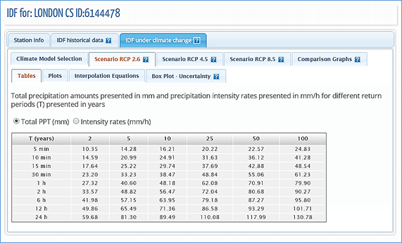
Figure 58. Updated IDF tables for future climate conditions – total precipitation in mm
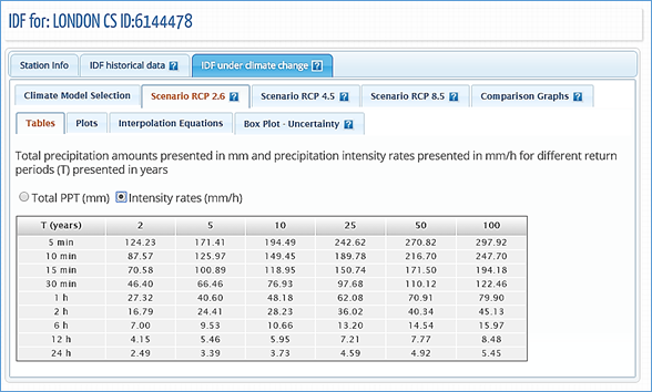
Figure 59. Updated IDF tables for future climate conditions – rainfall intensity in mm/h
2) Plots: the plots or graphs are also available for total precipitation (in mm) and rainfall intensity (mm/h) as presented in Figure 60 and Figure 61, respectively. The user can hide or show the IDF curve for each return period by clicking on individual return periods in the legend below the graph. Zoom is also available and is performed by dragging out a rectangle in the chart with the mouse pointer. The area selected is zoomed-in (Figure 50) and a “Reset zoom” button will be visible. The “Reset zoom” option will revert the zoom level to the original state. By hovering the mouse pointer over dots, the user can view precipitation, intensity and duration values for each point on the plot. The dots are calculated IDF values and the lines are plotted using the fitted equation that is presented under “Interpolation Equations” tab.
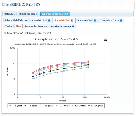
Figure 60. Total precipitation (in mm) updated IDF graph for different return periods
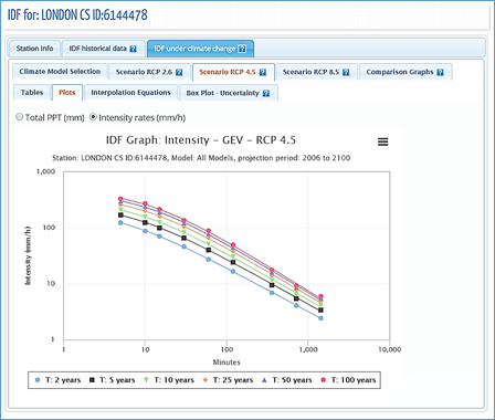
Figure 61. Rainfall intensity (in mm/h) updated IDF graph for different return periods
3) “Interpolation Equations”: an optimization algorithm is used to fit equations to the calculated IDF values. The equations are presented under the “Interpolation Equations” Tab as shown in Figure 62. Three coefficients A, B and t0 are calculated by the optimization algorithm for each return period (T) and presented as a table in Figure 62. This equation can be applied as and expedite method for interpolation and calculation for design storms.
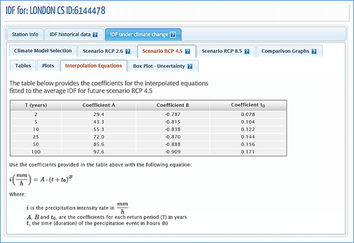
Figure 62. Fitted IDF equation for future scenario
4) Box Plot Uncertainty: Users can quickly view the distribution of results produced by each of the GCMs available within the tool by selecting the “Box Plot – Uncertainty” tab when generating future IDF curves using the “All Models” GCM option. Figure 63 provides an example of an uncertainty plot output. The plot was generated for the London CS rain station, using the “All Models” GCM option for the period 2006-2100, RCP 2.6. The plot indicates the range of values generated for each of the GCM datasets for this future scenario. See the Figure 64 for illustration of how to read the Box Plots.
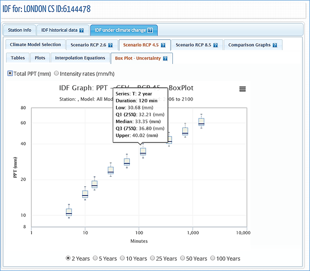
Figure 63. Box Plot – Uncertainty
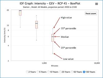
Figure 64. Reading Box Plots
5) Comparison Graphs: this option presents the summary and comparison between the IDF based on historical data and the median IDF for future periods (RCP 2.6, 4.5 and 8.5) as shown in Figure 65. The graphs are presented for each return period, i.e.: 2, 5, 10, 25, 50 and 100 years. The dots in Figure 65 represent the IDF table and the lines are plotted from the Interpolation Equations.
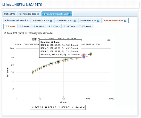
Figure 65. IDF comparison graphs
4 Review of IDF Updating Procedures
The IDF_CC tool version 3 offers three ways to obtain the updated IDFs for future climatic conditions based on the selected GCMs. The first and more direct way is to use an existing ECCC station. The user should follow the three easy steps to update the IDF for future climatic conditions as illustrated in Figure 66: 1) select one station, either from the map or from the list of stations; 2) calculate the IDF curves using the historical data (intermediate step) that can be used for comparison with the updated IDF for the future climatic conditions; and 3) select the GCM and projection period and generate updated IDF curves for future climatic conditions.
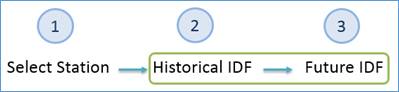
Figure 66. Updating IDFs for future climatic conditions for an ECCC station
The second option includes one additional step where the user creates their own station by providing information and data as shown in Figure 67. The remaining steps are the same as in the previous option.
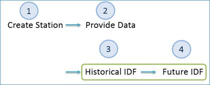
Figure 67. Updating IDF for future climatic conditions for a user-created station
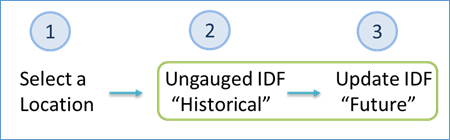
Figure 68. Updating IDFs for future climatic conditions for a selected location within Canada (Ungauged IDFs)
5 Final Comments
This report presents the User’s Manual for the Computerized IDF_CC tool for the Development of Intensity-Duration-Frequency-Curves Under a Changing Climate Version 3. It aims to assist in the updating of IDF curves for future climatic conditions. The IDF_CC tool uses a sophisticated though efficient methodology that incorporates changes in the distributional characteristics of GCMs between the baseline period and the projection period. The IDF_CC tool is easy to use and radically simplifies the IDF update process by automating very demanding procedures like downloading, extracting and manipulating data from various GCMs. The IDF_CC tool’s website www.idf-cc-uwo.ca should be regularly visited for the latest updates of the IDF_CC tool, new functionalities and updated documentation.
Acknowledgments
The authors would like to acknowledge the financial support by the Canadian Water Network Project under the Evolving Opportunities for Knowledge Application Grant to the second author for the initial phase of the project, and the Institute for Catastrophic Loss Reduction for continuous support of this project.
References
Allan R.P, and B.J. Soden, (2008). Atmospheric warming and the amplification of precipitation extremes. Science 321: 1480–1484.
Barnett D.N., S.J. Brown, J.M. Murphy, D.M.H. Sexton, and M.J. Webb, (2006). Quantifying uncertainty in changes in extreme event frequency in response to doubled CO2 using a large ensemble of GCM simulations. Climate Dynamics 26(5): 489–511, DOI: 10.1007/S00382-005-0097-1.
IPCC, (2013). Summary for Policymakers. In: Climate Change 2013: The Physical Science Basis. Contribution of Working Group I to the Fifth Assessment Report of the Intergovernmental Panel on Climate Change [Stocker, T.F., D. Qin, G.-K. Plattner, M. Tignor, S.K. Allen, J. Boschung, A. Nauels, Y. Xia, V. Bex and P.M. Midgley (eds.)]. Cambridge University Press, Cambridge, United Kingdom and New York, NY, USA.
Pacific Climate Impacts Consortium (PCIC), (2013). Statistically downscaled climate scenarios, https://pacificclimate.org/data/statistically-downscaled-climate-scenarios last accessed July 15, 2017.
Sandink, D., S.P. Simonovic, A. Schardong, and R. Srivastav, (2016) A Decision Support System for Updating and Incorporating Climate Change Impacts into Rainfall Intensity-Duration-Frequency Curves: Review of the Stakeholder Involvement Process, Environmental Modelling & Software Journal, 84:193-209.
Simonovic, S.P., A. Schardong, D. Sandink, and R. Srivastav, (2016) A Web-based Tool for the Development of Intensity Duration Frequency Curves under Changing Climate, Environmental Modelling & Software Journal, 81:136-153.
Solaiman, T.A. and S.P. Simonovic, (2011). Development of Probability Based Intensity-Duration Frequency Curves under Climate Change. Water Resources Research Report no. 072, Facility for Intelligent Decision Support, Department of Civil and Environmental Engineering, London, Ontario, Canada, 89 pp. ISBN: (print) 978-0-7714-2893-7; (online) 978-0-7714-2900-2.
Solaiman, T.A., L.M. King, and S.P. Simonovic, (2011), Extreme precipitation vulnerability in the Upper Thames River basin: uncertainty in climate model projections. Int. J. Climatol., 31: 2350–2364. doi:10.1002/joc.2244
Srivastav, R.K., A. Schardong., and S.P. Simonovic, (2014) Equidistance Quantile Matching Method for Updating IDF Curves under Climate Change, Water Resources Management. DOI 10.1007/s11269-014-0626-y.
Storn, R. and K. Price, (1997) ‘Differential Evolution - A Simple and Efficient Heuristic for Global Optimization over Continuous Spaces’, Journal of Global Optimization, 11, pp. 341–359.
Wilcox, E.M., Donner LJ., (2007) The frequency of extreme rain events in satellite rain-rate estimates and an atmospheric general circulation model. Journal of Climate 20(1): 53–69.
Vasan A., (2008) Optimization Using Differential Evolution. Water Resources Research Report no. 060, Facility for Intelligent Decision Support, Department of Civil and Environmental Engineering, London, Ontario, Canada, 38 pp.
Appendix - A: Papers/Reports on Differential Evolution - DE
Vasan A. (2008) - Optimization Using Differential Evolution. Water Resources Research Report no. 060, Facility for Intelligent Decision Support, Department of Civil and Environmental Engineering, London, Ontario, Canada, 38 pp:
http://www.eng.uwo.ca/research/iclr/fids/publications/products/60.pdf
Storn, R. and Price, K. (1997), ‘Differential Evolution - A Simple and Efficient Heuristic for Global Optimization over Continuous Spaces’, Journal of Global Optimization, 11, pp. 341–359.
http://link.springer.com/article/10.1023%2FA%3A1008202821328
Appendix - B: Previous reports in the Series
ISSN: (Print) 1913-3200; (online) 1913-3219
In addition to 78 previous reports (No. 01 – No. 78) prior to 2012
Samiran Das and Slobodan P. Simonovic (2012). Assessment of Uncertainty in Flood Flows under Climate Change. Water Resources Research Report no. 079, Facility for Intelligent Decision Support, Department of Civil and Environmental Engineering, London, Ontario, Canada, 67 pages. ISBN: (print) 978-0-7714-2960-6; (online) 978-0-7714-2961-3.
Rubaiya Sarwar, Sarah E. Irwin, Leanna King and Slobodan P. Simonovic (2012). Assessment of Climatic Vulnerability in the Upper Thames River basin: Downscaling with SDSM. Water Resources Research Report no. 080, Facility for Intelligent Decision Support, Department of Civil and Environmental Engineering, London, Ontario, Canada, 65 pages. ISBN: (print) 978-0-7714-2962-0; (online) 978-0-7714-2963-7.
Sarah E. Irwin, Rubaiya Sarwar, Leanna King and Slobodan P. Simonovic (2012). Assessment of Climatic Vulnerability in the Upper Thames River basin: Downscaling with LARS-WG. Water Resources Research Report no. 081, Facility for Intelligent Decision Support, Department of Civil and Environmental Engineering, London, Ontario, Canada, 80 pages. ISBN: (print) 978-0-7714-2964-4; (online) 978-0-7714-2965-1.
Samiran Das and Slobodan P. Simonovic (2012). Guidelines for Flood Frequency Estimation under Climate Change. Water Resources Research Report no. 082, Facility for Intelligent Decision Support, Department of Civil and Environmental Engineering, London, Ontario, Canada, 44 pages. ISBN: (print) 978-0-7714-2973-6; (online) 978-0-7714-2974-3.
Angela Peck and Slobodan P. Simonovic (2013). Coastal Cities at Risk (CCaR): Generic System Dynamics Simulation Models for Use with City Resilience Simulator. Water Resources Research Report no. 083, Facility for Intelligent Decision Support, Department of Civil and Environmental Engineering, London, Ontario, Canada, 55 pages. ISBN: (print) 978-0-7714-3024-4; (online) 978-0-7714-3025-1.
Roshan Srivastav and Slobodan P. Simonovic (2014). Generic Framework for Computation of Spatial Dynamic Resilience. Water Resources Research Report no. 085, Facility for Intelligent Decision Support, Department of Civil and Environmental Engineering, London, Ontario, Canada, 81 pages. ISBN: (print) 978-0-7714-3067-1; (online) 978-0-7714-3068-8.
Angela Peck and Slobodan P. Simonovic (2014). Coupling System Dynamics with Geographic Information Systems: CCaR Project Report. Water Resources Research Report no. 086, Facility for Intelligent Decision Support, Department of Civil and Environmental Engineering, London, Ontario, Canada, 60 pages. ISBN: (print) 978-0-7714-3069-5; (online) 978-0-7714-3070-1.
Sarah Irwin, Roshan Srivastav and Slobodan P. Simonovic (2014). Instruction for Watershed Delineation in an ArcGIS Environment for Regionalization Studies.Water Resources Research Report no. 087, Facility for Intelligent Decision Support, Department of Civil and Environmental Engineering, London, Ontario, Canada, 45 pages. ISBN: (print) 978-0-7714-3071-8; (online) 978-0-7714-3072-5.
Andre Schardong, Roshan K. Srivastav and Slobodan P. Simonovic (2014). Computerized Tool for the Development of Intensity-Duration-Frequency Curves under a Changing Climate: Users Manual v.1. Water Resources Research Report no. 088, Facility for Intelligent Decision Support, Department of Civil and Environmental Engineering, London, Ontario, Canada, 68 pages. ISBN: (print) 978-0-7714-3085-5; (online) 978-0-7714-3086-2.
Roshan K. Srivastav, Andre Schardong and Slobodan P. Simonovic (2014). Computerized Tool for the Development of Intensity-Duration-Frequency Curves under a Changing Climate: Technical Manual v.1. Water Resources Research Report no. 089, Facility for Intelligent Decision Support, Department of Civil and Environmental Engineering, London, Ontario, Canada, 62 pages. ISBN: (print) 978-0-7714-3087-9; (online) 978-0-7714-3088-6.
Roshan K. Srivastav and Slobodan P. Simonovic (2014). Simulation of Dynamic Resilience: A Railway Case Study. Water Resources Research Report no. 090, Facility for Intelligent Decision Support, Department of Civil and Environmental Engineering, London, Ontario, Canada, 91 pages. ISBN: (print) 978-0-7714-3089-3; (online) 978-0-7714-3090-9.
Nick Agam and Slobodan P. Simonovic (2015). Development of Inundation Maps for the Vancouver Coastline Incorporating the Effects of Sea Level Rise and Extreme Events. Water Resources Research Report no. 091, Facility for Intelligent Decision Support, Department of Civil and Environmental Engineering, London, Ontario, Canada, 107 pages. ISBN: (print) 978-0-7714-3092-3; (online) 978-0-7714-3094-7.
Sarah Irwin, Roshan K. Srivastav and Slobodan P. Simonovic (2015). Instructions for Operating the Proposed Regionalization Tool "Cluster-FCM" Using Fuzzy C-Means Clustering and L-Moment Statistics. Water Resources Research Report no. 092, Facility for Intelligent Decision Support, Department of Civil and Environmental Engineering, London, Ontario, Canada, 54 pages. ISBN: (print) 978-0-7714-3101-2; (online) 978-0-7714-3102-9.
Bogdan Pavlovic and Slobodan P. Simonovic (2016). Automated Control Flaw Generation Procedure: Cheakamus Dam Case Study. Water Resources Research Report no. 093, Facility for Intelligent Decision Support, Department of Civil and Environmental Engineering, London, Ontario, Canada, 78 pages. ISBN: (print) 978-0-7714-3113-5; (online) 978-0-7714-3114-2.
Sarah Irwin, Slobodan P. Simonovic and Niru Nirupama (2016). Introduction to ResilSIM: A Decision Support Tool for Estimating Disaster Resilience to Hydro-Meteorological Events. Water Resources Research Report no. 094, Facility for Intelligent Decision Support, Department of Civil and Environmental Engineering, London, Ontario, Canada, 66 pages. ISBN: (print) 978-0-7714-3115-9; (online) 978-0-7714-3116-6.
Tommy Kokas, Slobodan P. Simonovic (2016). Flood Risk Management in Canadian Urban Environments: A Comprehensive Framework for Water Resources Modeling and Decision-Making. Water Resources Research Report no. 095. Facility for Intelligent Decision Support, Department of Civil and Environmental Engineering, London, Ontario, Canada, 66 pages. ISBN: (print) 978-0-7714-3117-3; (online) 978-0-7714-3118-0.
Jingjing Kong and Slobodan P. Simonovic (2016). Interdependent Infrastructure Network Resilience Model with Joint Restoration Strategy. Water Resources Research Report no. 096, Facility for Intelligent Decision Support, Department of Civil and Environmental Engineering, London, Ontario, Canada, 83 pages. ISBN: (print) 978-0-7714-3132-6; (online) 978-0-7714-3133-3.
Sohom Mandal, Patrick A. Breach and Slobodan P. Simonovic (2017). Tools for Downscaling Climate Variables: A Technical Manual. Water Resources Research Report no. 097, Facility for Intelligent Decision Support, Department of Civil and Environmental Engineering, London, Ontario, Canada, 95 pages. ISBN: (print) 978-0-7714-3135-7; (online) 978-0-7714-3136-4.
Andre Schardong, Slobodan P. Simonovic and Dan Sandink (2017). Computerized Tool for the Development of Intensity-Duration-Frequency Curves Under a Changing Climate: Technical Manual v.2.0. Water Resources Research Report no. 098, Facility for Intelligent Decision Support, Department of Civil and Environmental Engineering, London, Ontario, Canada, 58 pages. ISBN: (print) 978-0-7714-3144-9; (online) 978-0-7714-3145-6.